Table of Contents
ToggleMS Excel has always been a savior and it is almost the first love of every Data enthusiast. Though there are multiple Analytics tools available the spreadsheet program is one of the most essential things that every aspiring Data Analyst should learn. It’s not just about gathering data but also arranging them in a proper manner that looks neat and presentable. This article will help you with 5 such Excel formulae that you will need if you’re looking for a Data Analyst profession.

MS Excel Functions and Their Advantage
1. CONCATENATE
This is a simple one. Let’s say you have two or more cells and another column or row will be the merge or combination of those two cells. This way of merging those cells to get a combined one using a certain formula is called Concatenate. You can use a maximum of 255 strings or 8192 characters in a concatenate formula but you cannot use an array such as C1:C20.

In this table, you can see that column B has the title ‘First Name’ and column C has ‘Last Name’. The next column D combines columns B and C and the title is ‘Full Name’. So combine the first and the last name using this formula:
=CONCATENATE(B4,” “,C4)
2. VLOOKUP
This formula works best when you want to search for any data that is arranged in a vertical column.

In this image, you can see how we have used VLOOKUP. There are a total of 3 columns where three separate data sets are present. Now let’s try to find the vertical data corresponding to the ID number 300 using VLOOKUP.
For that, you first need to move to a different cell and make a heading as VLOOKUP. Right on its left cell, write Search Value. Now, the search value is the ID against which we’re trying to find the corresponding vertical data. In the cell below the VLOOKUP title, we’ll start working on the formula.
- We’ll start with =VLOOKUP(
- Next, click on the cell where you want to get the result, that is in this case, F6 (right below the VLOOKUP cell).
- Then add a comma, and choose the entire matrix which in our case ranges from B3 to D8.
- Add another comma and then write the number of columns present in the entire data set which in our case is 3
- And then close the bracket.
Therefore, the entire formula looks like:
=VLOOKUP(F6,B3:D8,3)
The result is 110,000 which is exactly the vertical data (salary) corresponding to the ID number 300.
3. SUMIF
This is another important Excel formula that gives you the combined value of different cells but it is based on a certain criterion. When it comes to a large data set with multiple different numbers, you may not always want to get a combined value of all the cells. SUMIF allows you to get your desired result amidst the huge data. This is essential for complex data analysis.
Let’s see how you can use SUMIF to obtain the data you are looking for. In the above illustration, you can see that there are various types of columns and another two separate columns ‘Output’ and ‘Formula’. So once you’re done with writing the data, choose any different cell and write ‘Formula’. Under this cell, we’ll be calculating the value using SUMIF.
- The formula starts with, =SUMIF(
- Now you have to choose the data set corresponding to which you have to choose the value. In this case, you have to select the entire range from B2:B9, i.e., the column with the name ‘Sponsorship’.
- The next step is very crucial. In this section, we’ll choose the criterion barring which we want the result. Since the first criterion is with less/greater than operators and over here the operator is 25. So the formula is SUMIF(B2:B9,’<25’)
- Now for the other operators, you will have to choose a different range.
4. MINIFS/MAXIFS
This convenient equation not only discerns the lowest and highest values but also arranges them according to specific criteria. For instance, it can be applied to organize the ages of men and women in a sample, showcasing the values categorized by gender, thereby serving a dual purpose.

In the above example, you can see a cell highlighted in green that shows the result of 100. We wanted to find the lowest number corresponding to a salary is USD 56,000.
So the formula goes like this:
=MINIFS(B4:B14, C4:C13,56000)
5. COUNTIF
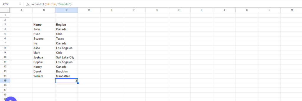
THE COUNTIFS formula counts the numbers of how many times a value appears based on one criterion. The image below shows how COUNTIF is used by Data Analysts when they have a large number of data but they’re looking for a particular parameter.

The first column under the title ‘Name’ has the name of the people and the next column ‘Region’ shows their hometown. In this scenario, we’re looking for how many people have their hometowns in Canada. Therefore, we have used the formula, =COUNTIF(C4:C14,”Canada”). You have to first select the entire that shows the hometown, i.e., the criterion we’re looking for and then have to mention the particular criterion we are seeking.
Conclusion
Now that you have got to know the Excel formulae that a Data Analyst often uses, you must start keeping track of these formulae. There are many other Excel formulae that Data Analysts use and if you want to know more about them, please drop your comment and share your feedback with us.

